bacondecomp

R package for understanding bias of TWFE in staggered settings

When the TWFE estimator is used in staggered DiD, the estimated \(\hat\tau_\text{TWFE}\) can be biased. The bacondecomp package decomposes the TWFE estimator and illustrates why it is biased. Documentation can be found here.

Install the packages as follows:

install.packages('bacondecomp')

---

sample code

Start by loading packages and data.

library(bacondecomp)
library(ggplot2)    # for plotting
library(readr)      # for importing data
df = read_csv('df.csv')

We start by breaking down the TWFE into its comparisions \(\hat\beta\) with bacon decomposition. We use the bacon() function to implement this:

decomp = bacon(
  formula   = outcome ~ treat,  # match TWFE variables
  data      = df,
  id_var    = "id",             # match TWFE fixed effect
  time_var  = "time"            # match TWFE fixed effect
)
decomp |> head()  # head() because a lot of comparisons

#>                       type  weight  avg_est
#> 1 Earlier vs Later Treated 0.14286 -2.45996
#> 2 Later vs Earlier Treated 0.14286 -8.48458
#> 3     Treated vs Untreated 0.71429 -2.66575
#>   treated untreated  estimate     weight                 type
#> 2      10     99999 -8.827665 0.03896104 Treated vs Untreated
#> 3       9     99999 -7.787725 0.06926407 Treated vs Untreated
#> 4       8     99999 -3.986033 0.09090909 Treated vs Untreated
#> 5       7     99999 -4.629684 0.10389610 Treated vs Untreated
#> 6       6     99999 -3.274153 0.10822511 Treated vs Untreated
#> 7       5     99999 -1.531851 0.10389610 Treated vs Untreated

We can see the top output is a summary of the general comparisons, while the bottom output is the top 6 rows of all the individual \(\hat\beta\) comparisons. We can also see Later vs. Earlier (already) treated is a comparison here, which is a forbidden comparison, biasing our estimates.

We can plot the estimates and weights of all the comparisons to better understand what each comparison’s value is, and how they are weighted.

decomp |>
  ggplot(aes(x = weight, y = estimate, shape = type, col = type)) +
  geom_point() +
  theme_light() +
  labs(
    x      = "Weights",
    y      = "Estimates",
    shape  = "Type",
    col    = "Type",
    title  = "Decomposition of TWFE"
  )

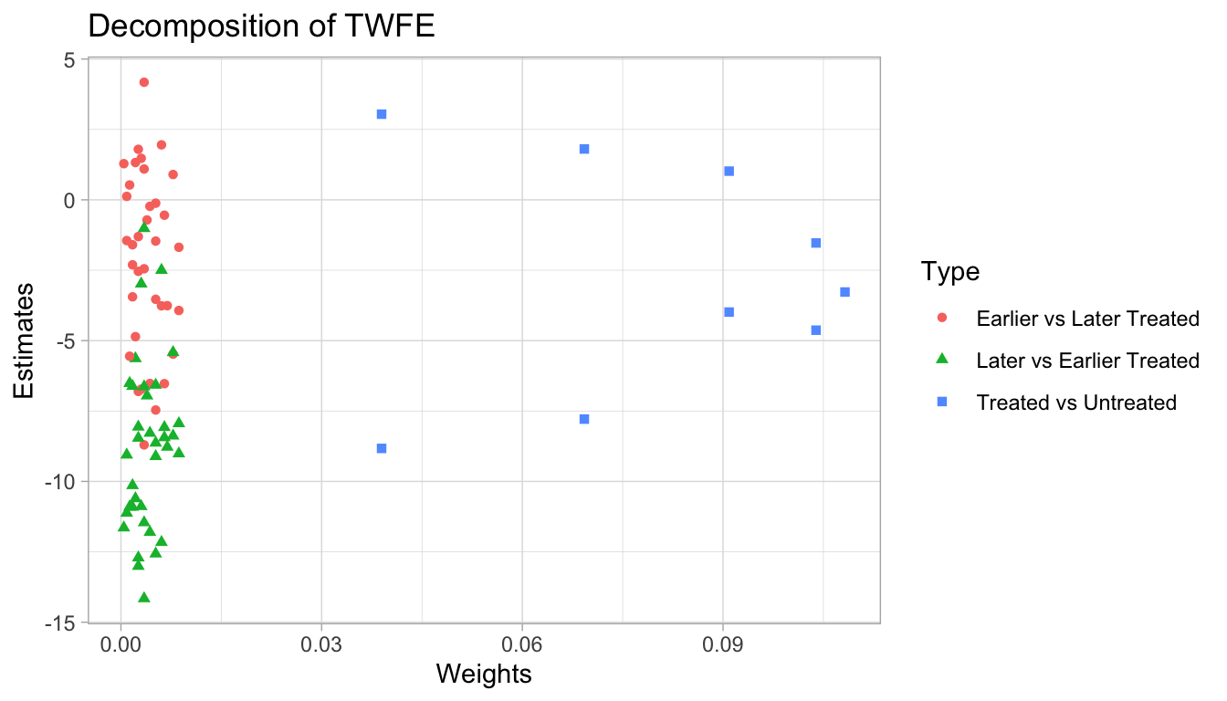
The green highlighted comparisons all involve earlier (already) treated units being used as control units, which is nonsensical. Bacon decomposition thus shows us the perils of relying on TWFE for staggered treatment.

We know that any negative weights of any comparisons \(\hat\beta\) are non-sensical. The graph also allows us to check this. In this example, there are no negative weights.