fixest

R package for TWFE and Interaction-Weighted (Sun and Abraham 2021)

fixest (and companion ggfixest) is a package for regressions targeted toward econometrics. For DiD, fixest allows the implementation of a basic TWFE model, as well as the Sun and Abraham (2021) interaction-weighted estimator. Documentation can be found here.

Install the package as follows:

install.packages('fixest')
install.packages('ggfixest')

---

sample code

Start by loading packages and the data:

library(fixest)
library(ggfixest)
library(readr)  # for importing data
df = read_csv('df.csv')

We use the feols() function to run the TWFE model.

mod = feols(
  fml   = outcome ~ treat + covar | id + time,  # covar is optional
  data  = df,                                   # your data
  vcov  = ~ id                                  # cluster SE by unit
)
mod |> summary()

#> OLS estimation, Dep. Var.: outcome
#> Observations: 950
#> Fixed-effects: id: 95,  time: 10
#> Standard-errors: Clustered (id) 
#>       Estimate Std. Error  t value  Pr(>|t|)    
#> treat -3.68310   0.361071 -10.2005 < 2.2e-16 ***
#> covar  1.01833   0.032416  31.4142 < 2.2e-16 ***
#> ---
#> Signif. codes:  0 '***' 0.001 '**' 0.01 '*' 0.05 '.' 0.1 ' ' 1
#> RMSE: 1.60906     Adj. R2: 0.691054
#>                 Within R2: 0.623425

We use the feols() function to run the TWFE event study for dynamic treatment effects.

mod = feols(
  fml   = outcome ~ i(rel.time, group, ref = -1) + covar | id + time,  # group = treat/never-treat
  data  = df,                                                          # your data
  vcov  = ~ id                                                         # cluster SE by unit
)
mod |> ggiplot(
  xlab    = "Time Relative to Treatment",  # x-axis label
  ylab    = "Dynamic ATT Estimate",        # y-axis label
  main    = "Dynamic Treatment Effects",   # title for plot
) +
  xlim(-8, 8) # select how many periods to display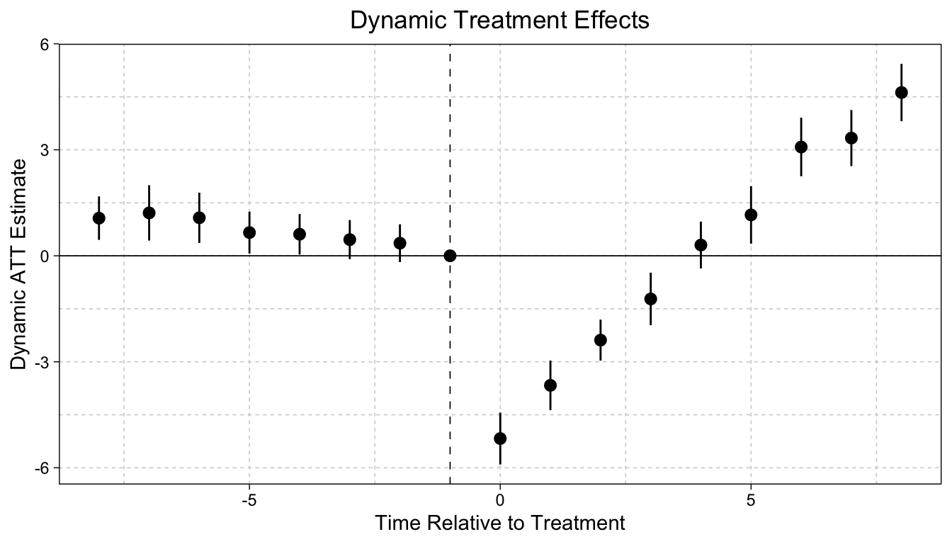

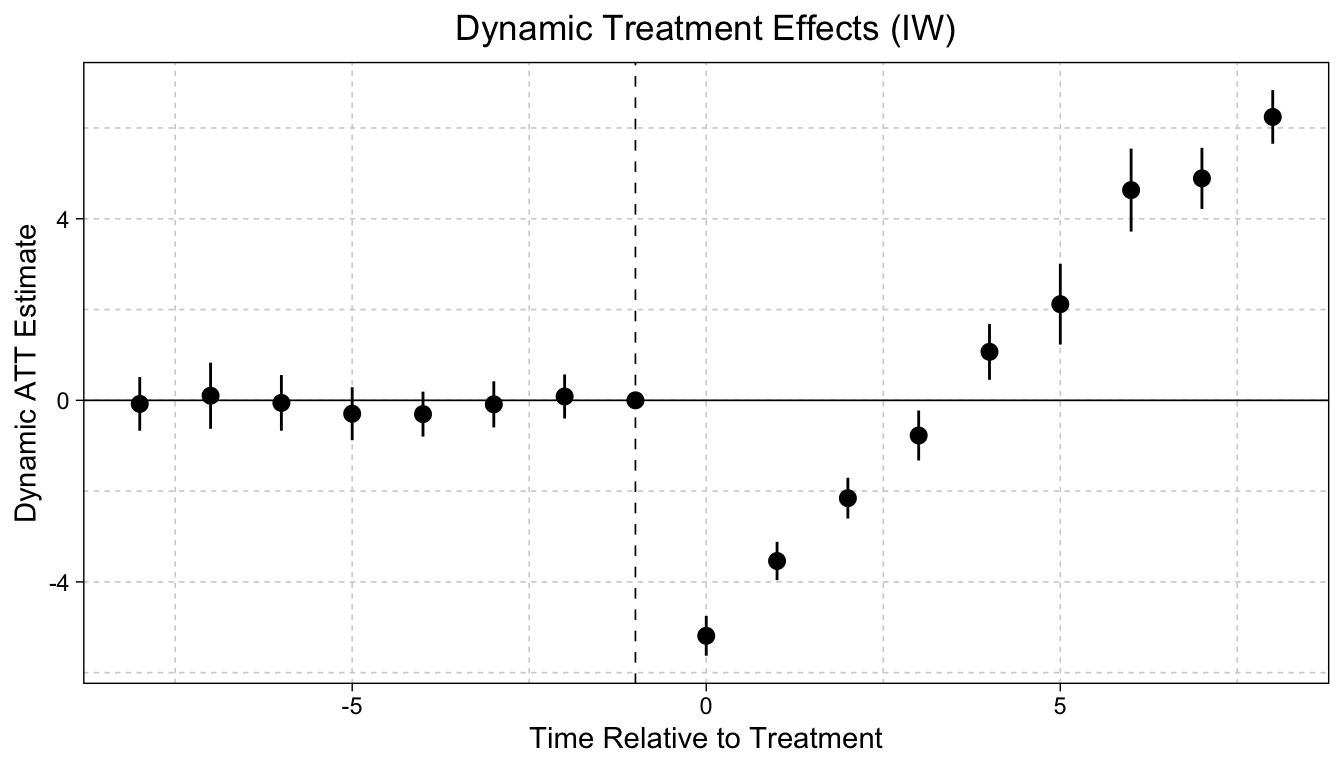
We add the sunab() function within feols() to implement the staggered DiD “Interaction-Weighted” estimator proposed by Sun and Abraham (2020).

Note: The cohort value for never-treated units should be a very large or very small number outside of the range of time.

mod = feols(
  fml = outcome ~ sunab(cohort, time) + covar | id + time,  # covar is optional
  data = df,
  vcov = ~ id                                               # clusters se by unit (id)
)
mod |>
  aggregate(agg  = "att") |>  # agg can also be "group" or "dynamic"
  print()

#>      Estimate Std. Error   t value     Pr(>|t|)
#> ATT -1.133749  0.2050705 -5.528584 2.882038e-07

And we can plot the Sun and Abraham event study using the ggiplot() function.

mod |> ggiplot(
  xlab    = "Time Relative to Treatment",       # x-axis label
  ylab    = "Dynamic ATT Estimate",             # y-axis label
  main    = "Dynamic Treatment Effects (IW)",   # title for plot
) + 
  xlim(-8, 8)                                   # how many periods to include.