didimputation

R package for the imputation estimator (Borusyak et al 2021)

didimputation is a package that implements the imputation DiD estimator proposed by Borusyak, Jaravel, and Speiss (2021) that solves the issues with TWFE in staggered settings. Documentation can be found here.

Install the package as follows:

install.packages('didimputation')

---

sample code

Start by loading packages and the data:

library(didimputation)
library(ggplot2)  # for plotting
library(readr)    # for importing data
df = read_csv('df.csv')

We use the did_imputation() function to run the model.

mod = did_imputation(
  data         = df,
  yname        = "outcome",
  gname        = "cohort",
  tname        = "time",
  idname       = "id",
  first_stage  = ~ covar | id + time  # can delete entire arg if no covars
)

mod |> print()

#> # A tibble: 1 × 6
#>   lhs     term  estimate std.error conf.low conf.high
#>   <chr>   <chr>    <dbl>     <dbl>    <dbl>     <dbl>
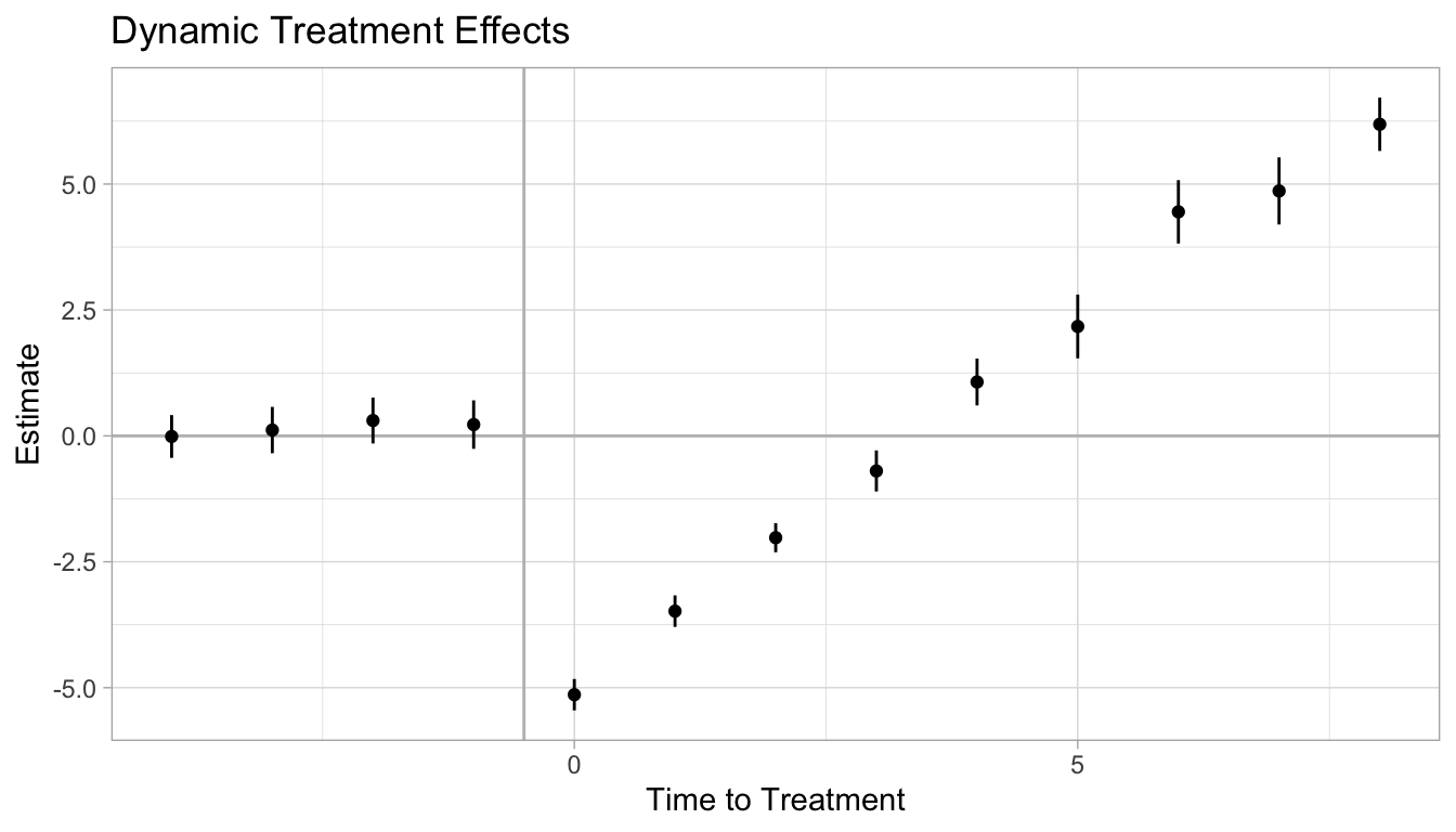
#> 1 outcome treat    -1.09     0.127    -1.34    -0.842

We can also estimate event-study dynamic effects for pre and post-treatment periods.

mod = did_imputation(
  data         = df,
  yname        = "outcome",
  gname        = "cohort",
  tname        = "time",
  idname       = "id",
  first_stage  = ~ covar | id + time,  # can delete entire arg if no covars
  horizon = T,                         # do not change
  pretrends = -4:-1                    # how many pre-treatment period to include
)

There is no simple built-in plot function for the package, so we will need to manually create a ggplot.

# convert output into table
tbl = mod |> as.data.table()

# filter for only treatment coefficients
tbl$term = tbl$term |> as.numeric()
tbl = tbl |> na.omit()

# ggplot
tbl |>
  ggplot(aes(x = term, y = estimate)) +
  geom_vline(xintercept = -0.5, color = "gray") +
  geom_hline(yintercept = 0, color = "gray") +
  geom_point() +
  geom_linerange(aes(ymin = conf.low, ymax = conf.high)) + 
  labs(title = "Dynamic Treatment Effects") +
  xlab("Time to Treatment") +
  ylab("Estimate") +
  theme_light()