pyfixest

Python package for TWFE, 2-stage DiD (Gardner 2021), and interaction-weighted (Sun and Abraham 2021).

pyfixest is a port of the fixest package for python, with slighty different syntax and offerings. pyfixest can implement the standard TWFE estimator for difference-in-differences. Documentation can be found here.

Install the package by inputting the following into the terminal:

pip install -U pyfixest

---

sample code

Start by loading packages and the data:

import pyfixest as pf
import pandas as pd
import numpy as np
import matplotlib.pyplot as plt
df = pd.read_csv('df.csv')

We can use the pf.feols() function to run the TWFE estimation for the ATT:

mod = pf.feols(
  fml   = "outcome ~ treat + covar | id + time",
  data  = df,
  vcov  = {"CRV1": "id"},  # change "id", do not touch "CRV1"
)
mod.summary()

#> ###
#> 
#> Estimation:  OLS
#> Dep. var.: outcome, Fixed effects: id+time
#> Inference:  CRV1
#> Observations:  950
#> 
#> | Coefficient   |   Estimate |   Std. Error |   t value |   Pr(>|t|) |   2.5% |   97.5% |
#> |:--------------|-----------:|-------------:|----------:|-----------:|-------:|--------:|
#> | treat         |     -3.683 |        0.361 |   -10.200 |      0.000 | -4.400 |  -2.966 |
#> | covar         |      1.018 |        0.032 |    31.414 |      0.000 |  0.954 |   1.083 |
#> ---
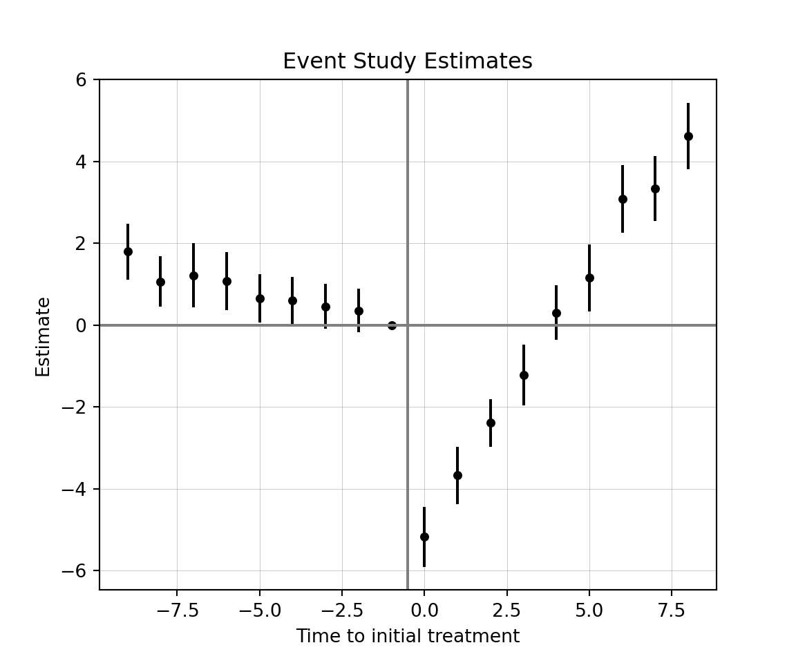
#> RMSE: 1.609 R2: 0.725 R2 Within: 0.623

Dynamic treatment effects for a TWFE event study can be calculated as follows:

mod = pf.feols(
  fml   = "outcome ~ i(rel_time, group, ref = -1) + covar | id + time",
  data  = df,
  vcov  = {"CRV1": "id"},  # change "id", do not touch "CRV1"
)

The iplot option within pyfixest is flawed, so we will have to manually plot them with matplotlib.

# save the results into tidy
res = mod.tidy()

# drop covariates from result dataframe (if required)
res = res.drop('covar')

# select needed columns
res = res[['Estimate', '2.5%', '97.5%']]

# no t=-1 estimate, so we will need to add it
new = pd.DataFrame({
    'Estimate': [0.00],
    '2.5%': [0.00],
    '97.5%': [0.00]
})
pre = res.iloc[:8]  # split dataframe so only pre-treat
post = res.iloc[8:]  # split dataframe so only post-treat
plot_df = pd.concat([pre, new, post], ignore_index = True)  # stick t=-1 between pre and post

# rel_time variable
rel_time = np.arange(-9, 9, dtype=np.int64)
plot_df['rel_time'] = rel_time  # add to dataframe

# plotting time
x = plot_df['rel_time']
y = plot_df['Estimate']
yerr = [y - plot_df['2.5%'], plot_df['97.5%'] - y]  # err distances

fig, ax = plt.subplots()
ax.scatter(x, y, color = "black", s = 15)  # s is for size
ax.errorbar(x, y, yerr = yerr, fmt = 'none', color = 'black', ecolor = 'black', capsize = 0)
ax.axvline(x = -0.5, color = "gray")
ax.axhline(y = 0, color = "gray")
ax.grid(True, linewidth = 0.3, alpha = 0.5, color = "gray")
ax.set_title('Event Study Estimates')
ax.set_xlabel('Time to initial treatment')
ax.set_ylabel('Estimate')
plt.show()