fect

R package for imputation estimators FEct, IFEct, and MC (Liu et al 2024)

fect is a package that implements imputation DiD estimators proposed by Liu, Xu, and Wang (2024) that solves the bias of the TWFE estimator in staggered and non-absorbing DiD. fect also includes modern estimators (ifect, mc) that are semi-robust against parallel trends violations. Documentation can be found here.

Install the package as follows:

install.packages('fect')

---

sample code

Start by loading packages and the data:

library(fect)
library(readr)  # for importing data
df = read_csv('df.csv')

Use the fect() function to estimate models. To switch between the models, alter the method = argument.

You should generally start with fect, then see if parallel trends is met, before going to ifect and mc. If you use ifect and mc, set CV = T.

mod = fect(
  formula  = outcome ~ treat + covar,  # covar is optional
  data     = df,
  index    = c("id", "time"),          # unit and time var
  method   = "fe",                     # use "fe", "ife", or "mc"
  CV       = F,                        # change to T for "ife" or "mc"
  se       = T,                        # don't change
  nboots   = 40,                       # usually you should use 200, larger is slower
  seed     = 1239                      # any number will work
)

mod |> print()

#> Call:
#> fect.formula(formula = outcome ~ treat + covar, data = df, index = c("id", 
#>     "time"), CV = F, method = "fe", se = T, nboots = 40, seed = 1239)
#> 
#> ATT:
#>                              ATT   S.E. CI.lower CI.upper   p.value
#> Tr obs equally weighted   -1.091 0.4746   -2.022  -0.1611 2.148e-02
#> Tr units equally weighted -2.964 0.5814   -4.104  -1.8246 3.432e-07
#> 
#> Covariates:
#>        Coef    S.E. CI.lower CI.upper p.value
#> covar 1.004 0.02042   0.9643    1.044       0

The output contains two different ATT estimates. It is typically conventional to use the first one, Tr obs equally weighted, which weights each observation \(it\) equally (rather than the second which weights all \(i\) equally).

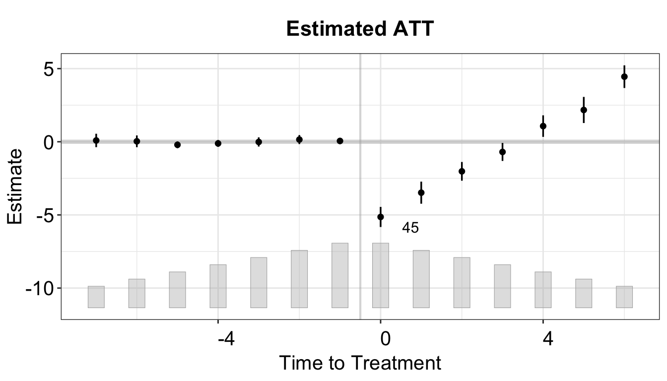
To plot dynamic effects, we use the plot() function.

mod |> plot(
  start0  = T,                    # don't change
  main    = NULL,                 # title
  ylab    = "Estimate",           # y-axis label
  xlab    = "Time to Treatment",  # x-axis label
  xlim    = c(-7, 7)              # what time periods to include (offset by +1)
)

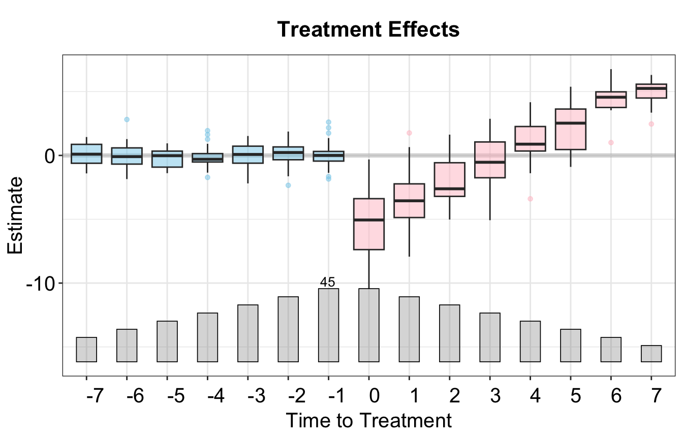
We can also plot the distributions of dynamic treatment effects as follows:

mod |> plot(
  start0  = T,                    # don't change
  type    = "box",                # don't change
  main    = NULL,                 # title
  ylab    = "Estimate",           # y-axis label
  xlab    = "Time to Treatment",  # x-axis label
  xlim    = c(-7, 7)              # what time periods to include (offset by +1)
)

The fect package contains an F-test and equivalence test to test parallel trends, accessed through plot():

mod |> plot(
  start0      = T,                    # don't change
  type        = "equiv",
  bound       = "equiv",
  pre.period  = c(-4, 0),             # how many pre-treat coef to test
  main        = NULL,                 # title
  ylab        = "Estimate",           # y-axis label
  xlab        = "Time to Treatment",  # x-axis label
  xlim        = c(-7, 7)              # what time periods to include (offset by +1)
)

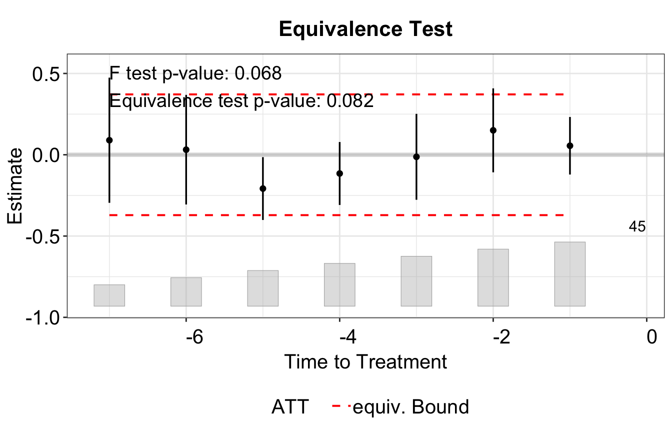
An F-test tests if the joint combination of pre-treatment coefficients is statistically significantly different than 0. Since we do not want the coefficients to be different than 0, we want to get a high p-value and fail to reject the null.

An Equivalence (TOST) test tests if the confidence intervals of our pre-treatment coefficients are within 0.36 standard deviations of the outcome variable of 0. Essentially, it tests if there is a substantively significant deviation in parallel trends.