DIDmultiplegtDYN

R package for DIDmultiple estimator (de Chaisemartin and D’Haultfœuille 2024)

DIDmultiplegtDYN is a package that implements the DIDmultiple estimator by de Chaisemartin and D’Haultfœuille (2024), that solves the issues with TWFE, handles non-absorbing and continuous treatments. Documentation can be found here.

Install the package as follows:

install.packages('DIDmultiplegtDYN')

---

sample code

Start by loading packages and the data:

library(DIDmultiplegtDYN)
library(ggplot2)  # for plotting
library(readr)    # for importing data
df = read_csv('df.csv')

We use the did_multiplegt_dyn() function to complete the estimation process.

If you have a continuous or quasi-continuous treatment, or are having issues, set continuous = 1. Covariates for conditional parallel trends are possible to include, but they are used differently, and may cause issues.

mod = did_multiplegt_dyn(
  # required arguments
  df          = df,
  outcome     = "outcome",
  group       = "id",       # Note: group here refers to unit, not cohort
  time        = "time",
  treatment   = "treat",
  effects     = 4,          # Number of post-treatment periods dynamic effects
  placebo     = 4,          # Number of pre-treatment periods of effects
  controls    = NULL,       # optional, vector (string) of covariates.
  continuous  = NULL,       # change to 1 if your treatment is true
  graph_off   = T
)

mod |> print()

#> 
#> ----------------------------------------------------------------------
#>        Estimation of treatment effects: Event-study effects
#> ----------------------------------------------------------------------
#>              Estimate SE      LB CI    UB CI    N   Switchers
#> Effect_1     -5.04943 0.45371 -5.93869 -4.16017 675 45       
#> Effect_2     -3.25734 0.49253 -4.22269 -2.29199 580 40       
#> Effect_3     -2.17826 0.54482 -3.24609 -1.11044 490 35       
#> Effect_4     -0.03749 0.50608 -1.02940 0.95442  405 30       
#> 
#> Test of joint nullity of the effects : p-value = 0.0000
#> ----------------------------------------------------------------------
#>     Average cumulative (total) effect per treatment unit
#> ----------------------------------------------------------------------
#>  Estimate        SE     LB CI     UB CI         N Switchers 
#>  -2.89921   0.38159  -3.64711  -2.15131       780       150 
#> Average number of time periods over which a treatment effect is accumulated: 2.3333
#> 
#> ----------------------------------------------------------------------
#>      Testing the parallel trends and no anticipation assumptions
#> ----------------------------------------------------------------------
#>              Estimate SE      LB CI    UB CI   N   Switchers
#> Placebo_1    0.27204  0.49208 -0.69242 1.23651 580 40       
#> Placebo_2    -0.72910 0.61928 -1.94287 0.48467 405 30       
#> Placebo_3    -0.27729 0.55098 -1.35720 0.80262 250 20       
#> Placebo_4    0.00895  1.00786 -1.96642 1.98433 115 10       
#> 
#> Test of joint nullity of the placebos : p-value = 0.5860
#> 
#> 
#> The development of this package was funded by the European Union.
#> ERC REALLYCREDIBLE - GA N. 101043899

The Estimation of treatment effects: Event-study effects are the post-treatment dynamic effects. The Average cumulative (total) effect per treatment unit is the ATT estimate. The Testing the parallel trends and no anticipation assumptions is the pre-treatment coefficient estimates.

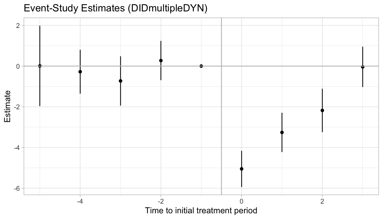
We can plot the dynamic treatment effects in a plot. The simplest way is to use the default plot - in the original model estimation within did_multiplegt_dyn(), set graph_off = equal to F.

However, the default plot is kind of ugly (in my opinion), and also does not use the conventional numbering of the initial treatment period (it uses t=1 as the initial treatment period). Thus, we can also manually create a ggplot:

# extract effects (the rev() function used because placebo effects are in the opposite order)
effects = c(rev(mod$results$Placebos[,1]), 0, mod$results$Effects[,1])  # extract pre/post effects
lwr = c(rev(mod$results$Placebos[,3]), 0, mod$results$Effects[,3])  # extract lower confint
upr = c(rev(mod$results$Placebos[,4]), 0, mod$results$Effects[,4]) # extract upper confint

# create rel.time variable matching number of pre/post periods
rel.time = c(-5:3)

# create plotting dataframe
plot.df = data.frame(rel.time, effects, lwr, upr)

# ggplot
plot.df |>
  ggplot(aes(x = rel.time, y = effects)) +
  geom_point() +
  geom_linerange(aes(ymin = lwr, ymax = upr)) +
  geom_hline(yintercept = 0, color = "gray") +
  geom_vline(xintercept = -0.5, color = "gray") +
  labs(title = "Event-Study Estimates (DIDmultipleDYN)") +
  xlab("Time to initial treatment period") +
  ylab("Estimate") +
  theme_light()