did

R package for doubly-robust and ipw DiD estimator (callaway and sant’anna 2021)

did is a package that implements the DiD estimators (doubly-robust, inverse probability weighting) proposed by Callaway and Sant’Anna (2021) that solves the bias of the TWFE estimator in staggered DiD. Documentation can be found here.

Install the package as follows:

install.packages('did')

---

sample code

Start by loading packages and the data:

# packages needed:
library(did)
library(readr)  # for importing data
df = read_csv('df.csv')

We use the att_gt() function to run the matching process of csdid. We can use the doubly-robust (dr) method, or the inverse probability weighing (ipw) method by changing the argument of est_method =.

Notes: id variable should be transformed to an integer variable before starting. Set cohort = 0 for never-treated units. Generally, doubly-robust is the better estimator, so use doubly-robust unless there is an error.

mod = att_gt(
  # required arguments
  yname                   = "outcome",
  tname                   = "time",
  idname                  = "id",            # must be a integer-variable
  gname                   = "cohort",        # cohort = 0 for never-treated
  est_method              = "dr",            # change to ipw if you are having issues
  base_period             = "universal",     # do not change
  allow_unbalanced_panel  = T,               # generally good to keep this T
  data                    = df,
  xformla                 = ~ covar,        # (optional)
  control_group           = "nevertreated",  # use "notyettreated" if sample size is small
  panel                   = T                # change to F if you are using rep. cross-section
)

We use the aggte() function to aggregate our matched treatment effects into an overall treatment effect.

mod |>
  aggte(type  = "simple", na.rm = T) |>
  summary(att)

#> 
#> Call:
#> aggte(MP = mod, type = "simple", na.rm = T)
#> 
#> Reference: Callaway, Brantly and Pedro H.C. Sant'Anna.  "Difference-in-Differences with Multiple Time Periods." Journal of Econometrics, Vol. 225, No. 2, pp. 200-230, 2021. <https://doi.org/10.1016/j.jeconom.2020.12.001>, <https://arxiv.org/abs/1803.09015> 
#> 
#> 
#>      ATT    Std. Error     [ 95%  Conf. Int.]  
#>  -1.1237        0.4887    -2.0815     -0.1659 *
#> 
#> 
#> ---
#> Signif. codes: `*' confidence band does not cover 0
#> 
#> Control Group:  Never Treated,  Anticipation Periods:  0
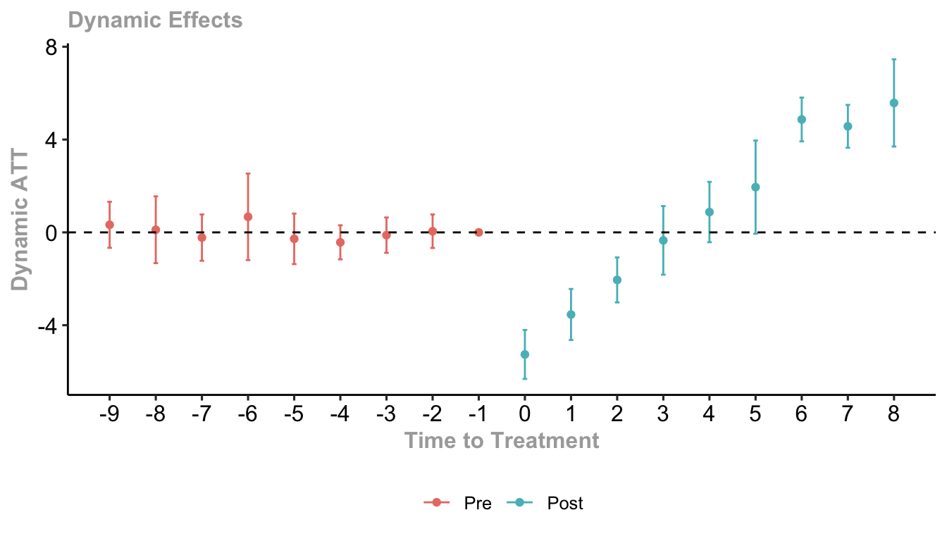
#> Estimation Method:  Doubly Robust

We can estimate dynamic treatment effects with the aggte() function and plot with the ggdid() function.

mod |>
  aggte(type   = "dynamic", na.rm  = T) |>
  ggdid(
    xlab    = "Time to Treatment",  # x-axis label
    ylab    = "Dynamic ATT",        # y-axis label
    title   = "Dynamic Effects"     # you can include a title string if you want
  )

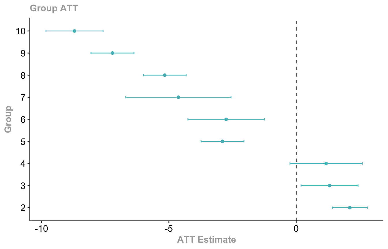
We can also aggregate effects by initial treatment period group, and with the ggdid() function:

mod |>
  aggte(type   = "group", na.rm  = T) |>
  ggdid(
    xlab    = "ATT Estimate",  # x-axis label
    ylab    = "Group",         # y-axis label
    title   = "Group ATT"      # you can include a title string if you want
  )

Other options for type = include "calendar", which displays the treatment effects grouped by actual (not relative) time period.