PanelMatch

R package for PanelMatch DiD estimator (Imai, Kim, and Wang 2023)

PanelMatch is a package that implements the PanelMatch estimator by Imai, Kim, and Wang (2023) that solves the bias of the TWFE estimator in staggered and non-absorbing DiD. Documentation can be found here.

Install the package as follows:

install.packages('PanelMatch')

---

sample code

Start by loading packages and the data:

library(PanelMatch)
library(readr)    # for importing data
library(ggplot2)  # for plotting
df = read_csv('df.csv')

PanelMatch requires us to pre-process the data with the PanelData() function:

Note: id variable should be transformed to an integer variable before starting.

# PanelMatch dislikes tidyverse df's, so do this:
df = df |> as.data.frame()

df.panel = PanelData(
  panel.data  = df,        # your data
  unit.id     = "id",      # your unit var (integer only)
  time.id     = "time",    # your time period var (integer only)
  treatment   = "treat",   # your treatment var
  outcome     = "outcome"  # your outcome var
)

Now, we can run the PanelMatch matching process with PanelMatch() to match based on lag-period pre-history:

Lag refers to periods before the treatment in which to match on. Leads refer to periods after the treatment on which to estimate.

match = PanelMatch(
  lag                = 3,              # number of pre-periods to match treat history
  panel.data         = df.panel,       # PanelData generated data
  lead               = c(0:6),         # how many post-treat dynamic effects to estimate
  qoi                = "att",
  refinement.method  = "mahalanobis",  # set to "none" if no covariates
  match.missing      = T,
  covs.formula       = ~ covar,        # (optional, can exclude)
  placebo.test       = T               # (optional, but may cause issues)
)

To aggregate all the matched comparisons into a singular ATT, we use the PanelEstimate() function.

match |>
  PanelEstimate(
    panel.data = df.panel,  # PanelData object
    pooled     = T,         # tells R to calculate ATT
    moderator  = NULL       # optional. character string for var to calculate heterogenous effects
  ) |>
  print()

#> Point estimates:
#> [1] 1.563779
#> 
#> Standard errors:
#> [1] 1.189761
#> 
#> Estimates produced with 5 observations (non-empty matched sets)

The Point estimates are the estimated ATT, and the standard errors are provided.

We can estimate event-study effects with the PanelEstimate() function for post-treatment effects, and the placebo_test() function for pre-treatment effects.

# estimate post-treatment effects
post = match |>
  PanelEstimate(
    panel.data = df.panel,  # PanelData object
    pooled     = F          # tells R to calculate dynamic effects
)

# estimate pre-treatment effects
pre = match |>
  placebo_test(
  panel.data = df.panel,  # PanelData object
  lag.in     = 3,         # should equal lag in PanelMatch()
  plot       = F
)

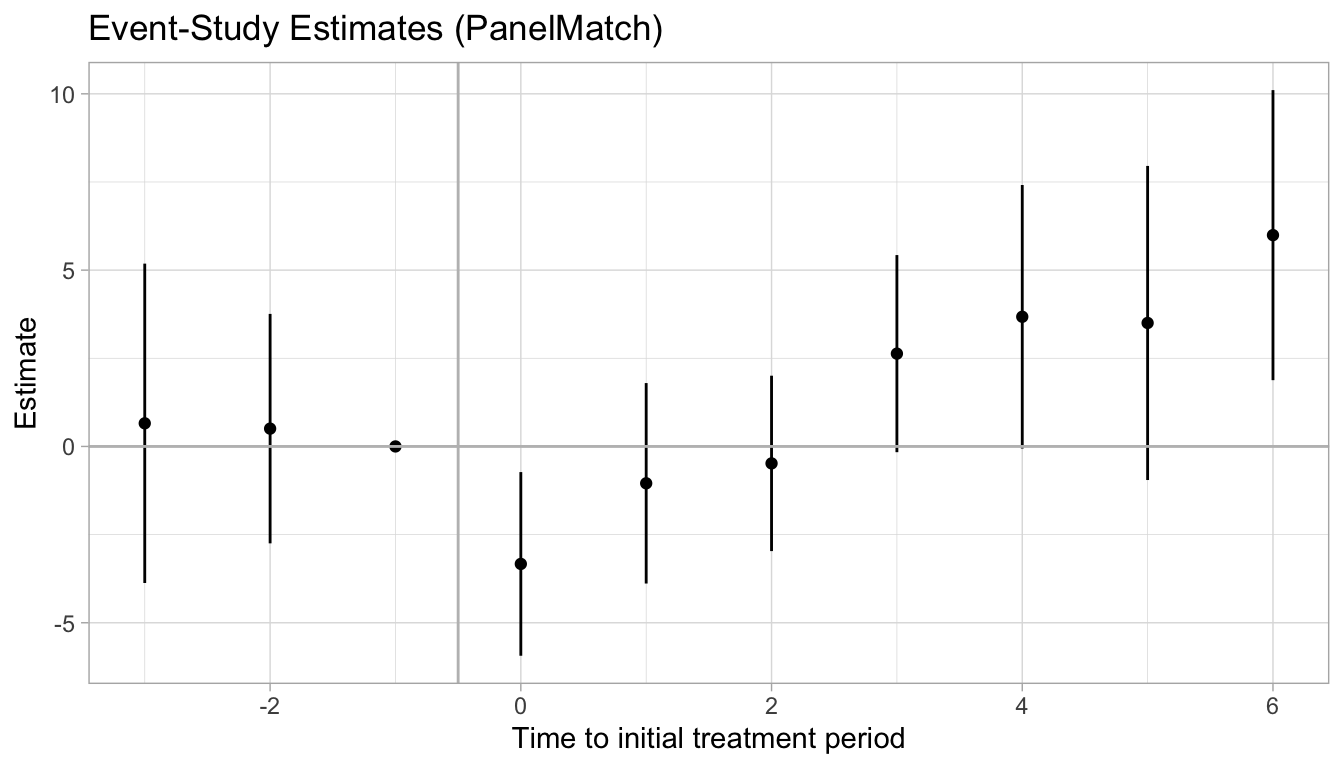
The built in plotting functions are lackluster, so we will create a manual ggplot to plot the results.

# combine pre and post estimates
effects = c(pre$estimate, 0, post$estimate)  # there is no t=-1 effect estimated so add it
se = c(pre$standard.error, 0, post$standard.error)

# create rel.time variable for pre/post periods
rel.time = c(-3:6)  

# create results df
results.df = data.frame(rel.time, effects, se)

# first create lwr and upr bounds for se
results.df$se.lwr = results.df$effects - 1.96*results.df$se
results.df$se.upr = results.df$effects + 1.96*results.df$se

results.df |>
  ggplot(aes(x = rel.time, y = effects)) +
  geom_point() +
  geom_linerange(aes(ymin = se.lwr, ymax = se.upr)) +
  geom_hline(yintercept = 0, color = "gray") +
  geom_vline(xintercept = -0.5, color = "gray") +
  labs(title = "Event-Study Estimates (PanelMatch)") +
  xlab("Time to initial treatment period") +
  ylab("Estimate") +
  theme_light()